Plastic Pollution 🚮

This week’s CorrelAid TidyTuesday Coding Hangout included a lot of casual chats and discussions about various #rstats topics, so not a lot of us managed to create a visualization (which is ok!). We still learned a lot and - most importantly during the current times - had fun and engaged with each other. We discussed different the advantages and disadvantages of the two most prominent blogging frameworks in R - blogdown and distill - and learned how to control the spacing between the dots in dotted lines: https://ggplot2.tidyverse.org/reference/aes_linetype_size_shape.html . 🤓

Here are the two contributions from this week:

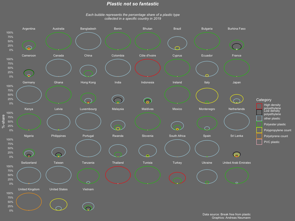
A bubble chart

by Andreas Neumann

library(tidyverse)
library(ggforce)
library(scales)
library(glue)
plastics <- readr::read_csv('https://raw.githubusercontent.com/rfordatascience/tidytuesday/master/data/2021/2021-01-26/plastics.csv')

###load data and transform into long data set###
b<-subset(plastics, year==2019 & parent_company=="Grand Total")
tall <- b %>% gather(key = total, value = cat, empty:pvc)
tall$id <- group_indices(tall, country)

## Warning: The `...` argument of `group_keys()` is deprecated as of dplyr 1.0.0.
## Please `group_by()` first
## This warning is displayed once every 8 hours.
## Call `lifecycle::last_warnings()` to see where this warning was generated.

tall<-tall%>%
  mutate_if(is.numeric, ~replace(., is.na(.), 0))
###add percentages+additional data wrangling###
tall<- tall %>% dplyr::group_by(id) %>% dplyr::mutate(percent = cat/sum(cat))
tall[which(tall$country=="Cote D_ivoire"),1] <- "Côte d'Ivoire"
tall[which(tall$country=="Taiwan_ Republic of China (ROC)"),1] <- "Taiwan"
tall[which(tall$country=="NIGERIA"),1] <- "Nigeria"
tall[which(tall$country=="ECUADOR"),1] <- "Ecuador"
tall[which(tall$country=="United States of America"),1] <- "United States"
###Plot###
tall%>%
  dplyr::filter(total!="empty")%>%
  dplyr::filter(country!="EMPTY")%>%
  #subset(percent!=1.0)%>%
  #subset(percent!=0.0)%>%
  dplyr::arrange(country,percent, .by_group = TRUE)%>%
  ggplot() +
  geom_circle(aes(x0=0, y0 =percent/2, r =percent/2,color=total),alpha=5)+
  facet_wrap(~country)+  
  scale_y_continuous(labels = percent,name="%-share")+
  scale_x_continuous(breaks=NULL)+
  scale_colour_manual(name="Category",values = c("red","black","lightblue","green3","yellow","orange","pink"), labels = c("High density\npolyethylene", "Low density\npolyethylene", "other plastic","Polyester plastic","Polypropylene count","Polystyrene count","PVC plastic"))+
  labs(title = "Plastic not so fantastic\n",subtitle = "Each bubble represents the percentage share of a plastic type\ncollected in a specific country in 2019\n",caption = glue("Data source: Break free from plastic\nGraphics: Andreas Neumann"))+
  theme(plot.title = element_text(color="white", size=14,hjust = 0.5, face="bold.italic"),
        axis.title.y = element_text(color = "white"),
        axis.title.x = element_blank(),
        axis.text.y = element_text(color = "white", size = 8),
        axis.ticks.y = element_blank(),
        axis.text.x = element_blank(),
        panel.grid.major = element_line(linetype = "blank"),
        panel.grid.minor = element_blank(),
        strip.background =element_rect(fill="gray48"),
        strip.text = element_text(colour = 'white'),
        panel.background = element_rect(fill = "gray48", color = NA),
        plot.background = element_rect(fill = "gray48", color = NA),
        plot.subtitle=element_text(size=10, hjust=0.5, face="italic", color="white"),
        legend.background = element_rect(fill = "gray48", color = NA),
        legend.text = element_text(color = "white"),
        legend.title = element_text(color = "white"),
        legend.key = element_rect(fill = "gray48"),
        title = element_text(colour = "white"))

Using CSS grids for Rmd layout

by Ihaddaden M. EL Fodil

Check out the full page here and the source code in this GitHub repository.